§ 1.7. Dual canonical projections.
Systematic investigations at Tübingen on long-range aperiodic
order started out from point symmetry forbidden in a periodic lattice and employ the dual cell geometry of
a lattice of dimension ![]() .
.
With my research group at Tübingen since 1982 I systematically explored the projection method from
an n-dimensional lattice ![]() .
.
A first central idea was to fix the
irrational section in Bohr's theory by the selection of a non-crystallographic point group.
Therefore the n-dimensional lattices were chosen such that they were compatible with a representation of a non-crystallographic point group
![]() .
The linear subspace
.
The linear subspace ![]() for the quasicrystal,
the irrational section according to Bohr, was then uniquely determined by
decomposing the representation of the point group into its irreducible parts. A subspace
for the quasicrystal,
the irrational section according to Bohr, was then uniquely determined by
decomposing the representation of the point group into its irreducible parts. A subspace ![]() with irreducible but non-crystallographic representation
with irreducible but non-crystallographic representation ![]() then
carries the construction of the quasicrystal structure.
To characterize this structure we employed the geometry of the lattice
then
carries the construction of the quasicrystal structure.
To characterize this structure we employed the geometry of the lattice
![]() and its projection to
and its projection to ![]() .
.
A second central idea of our analysis
was the notion of duality in this geometry.
We considered the geometry of high-dimensional Voronoi- or
Wigner-Seitz cells of ![]() , defined by all
points closer to a fixed lattice point than to any other one. The vertices of these Voronoi cells, called the holes of the lattice, form the centers of Delone cells dual to the Voronoi cells.
For the concept of holes in lattices we refer to [8].
We studied the hierarchy of m-dimensional boundaries,
, defined by all
points closer to a fixed lattice point than to any other one. The vertices of these Voronoi cells, called the holes of the lattice, form the centers of Delone cells dual to the Voronoi cells.
For the concept of holes in lattices we refer to [8].
We studied the hierarchy of m-dimensional boundaries, ![]() ,
abbreviated as m-boundaries, of both Voronoi and Delone cells associated with a lattice. We found that these boundaries admit a general notion of duality. Any m-boundary
,
abbreviated as m-boundaries, of both Voronoi and Delone cells associated with a lattice. We found that these boundaries admit a general notion of duality. Any m-boundary ![]() of a Voronoi cell can be described as
the intersection of the Voronoi cells for a finite set of lattice points.
This finite set of lattice points has a
convex hull of dimension (n-m).
We showed that this convex hull is a dual (n-m)-boundary denoted
as
of a Voronoi cell can be described as
the intersection of the Voronoi cells for a finite set of lattice points.
This finite set of lattice points has a
convex hull of dimension (n-m).
We showed that this convex hull is a dual (n-m)-boundary denoted
as ![]() , from a Delone cell.
This duality relation we took as a basis for the study of quasiperiodic tilings.
For m=0, the 0-boundaries of Voronoi cells are the holes of the lattice.
The duals to these 0-boundaries are precisely the Delone cells.
, from a Delone cell.
This duality relation we took as a basis for the study of quasiperiodic tilings.
For m=0, the 0-boundaries of Voronoi cells are the holes of the lattice.
The duals to these 0-boundaries are precisely the Delone cells.
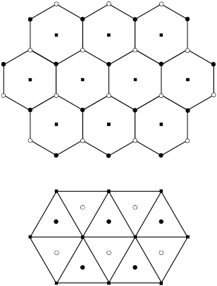
Example 2.3: Duality in the hexagonal lattice ![]() .
We illustrate duality in Fig. 5 for the root lattice
.
We illustrate duality in Fig. 5 for the root lattice ![]() .
Here we use the standard terminology of root lattices as given for example
in [8].
.
Here we use the standard terminology of root lattices as given for example
in [8].
A particular case of duality arises for hypercubic lattices ![]() in
in ![]() .
The Voronoi cells are hypercubes, and the holes form a second hypercubic lattice,
shifted from the vertices to the centers of the hypercubes. Duality still work, but there is no geometric distinction between Voronoi and Delone cells and tilings based on them.
This particular case appears already in the projection of the
Fibonacci tiling from
the square lattice
.
The Voronoi cells are hypercubes, and the holes form a second hypercubic lattice,
shifted from the vertices to the centers of the hypercubes. Duality still work, but there is no geometric distinction between Voronoi and Delone cells and tilings based on them.
This particular case appears already in the projection of the
Fibonacci tiling from
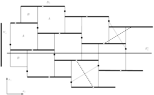
the square lattice ![]() , Fig. 6.
, Fig. 6.
Example 2.4: Scaling in the lattice ![]() :
For the Fibonacci projection we describe the scaling property of the
lattice
:
For the Fibonacci projection we describe the scaling property of the
lattice ![]() , compare [35]. First of all we write down in terms of two unit length orthogonal column vectors a basis matrix
, compare [35]. First of all we write down in terms of two unit length orthogonal column vectors a basis matrix![]() ,
,
![B=\left[\begin{array}[]{ll}-\sqrt{\frac{-\tau+3}{5}}&\sqrt{\frac{\tau+2}{5}}\\
\sqrt{\frac{\tau+2}{5}}&\sqrt{\frac{-\tau+3}{5}}\end{array}\right].](mi/mi101.png) |
(7) |
These two basis vectors connect a lattice point to two next neighbours (black squares) in Fig. 6.
The upper and lower row of ![]() describe the projections of the basis vectors
describe the projections of the basis vectors
![]() along the directions
along the directions ![]() in Fig. 6.
Now it can be checked that the basis matrix
in Fig. 6.
Now it can be checked that the basis matrix ![]() obeys the equation
obeys the equation
![\left[\begin{array}[]{ll}-\tau^{{-1}}&0\\
0&\tau\end{array}\right]\: B=B\;\left[\begin{array}[]{ll}1&1\\
1&0\end{array}\right].](mi/mi111.png) |
(8) |
The right-hand matrix multiplication describes a linear transformation
with determinant ![]() of the basis vectors with integer coefficients,
that is a symmetry transformation of the lattice
of the basis vectors with integer coefficients,
that is a symmetry transformation of the lattice ![]() . On the left-hand side,
this multiplication is expressed in the form of a scaling of the basis vectors
with scaling factors
. On the left-hand side,
this multiplication is expressed in the form of a scaling of the basis vectors
with scaling factors ![]() in the parallel and the perpendicular direction respectively. So the scaling in parallel space by
in the parallel and the perpendicular direction respectively. So the scaling in parallel space by ![]() can be interpreted as part of a transform of the lattice into itself. When this scaling is applied to the two original tiles of length
can be interpreted as part of a transform of the lattice into itself. When this scaling is applied to the two original tiles of length ![]() , it scales them into two tiles of length
, it scales them into two tiles of length ![]() .
The scaled tiles can be decomposed into the original tiles. By repeating this
scaling one can generate a Fibonacci string of arbitrary length. In any step of this generation, the frequency of occurence of each of the two tiles
is given by successive
/Fibonacci numbers.
.
The scaled tiles can be decomposed into the original tiles. By repeating this
scaling one can generate a Fibonacci string of arbitrary length. In any step of this generation, the frequency of occurence of each of the two tiles
is given by successive
/Fibonacci numbers.
We return to the general projection from a lattice. We found that, when ![]() becomes the dimension of the physical or parallel space
becomes the dimension of the physical or parallel space ![]() , this linear subspace is tiled by the parallel projections of m-boundaries
from Voronoi cells. The perpendicular projections to the complementary subspace
, this linear subspace is tiled by the parallel projections of m-boundaries
from Voronoi cells. The perpendicular projections to the complementary subspace
![]() plays an important role in the dual projection technique: it determines the so called windows of the objects. The role of a window in
plays an important role in the dual projection technique: it determines the so called windows of the objects. The role of a window in
![]() for the tiling on
for the tiling on ![]() is defined by the rule: Whenever
the irrational section
is defined by the rule: Whenever
the irrational section ![]() within
within ![]() hits a window for a tile in
hits a window for a tile in ![]() , the tile
will appear in the tiling. Specifically, if the tiling consists of parallel projections of m-boundaries say from Voronoi cells,
the windows for these tiles are the perpendicular projections of the
dual
, the tile
will appear in the tiling. Specifically, if the tiling consists of parallel projections of m-boundaries say from Voronoi cells,
the windows for these tiles are the perpendicular projections of the
dual ![]() -boundaries. The windows for the vertices of the
canonical tilings
-boundaries. The windows for the vertices of the
canonical tilings ![]() projected
from Voronoi or Delone cells, are the perpendicular
projections of the set of Delone cells and of Voronoi cells
of
projected
from Voronoi or Delone cells, are the perpendicular
projections of the set of Delone cells and of Voronoi cells
of ![]() respectively. Examples of vertex windows for the icosahedral tilings
are shown in Figs. 10, 11.
respectively. Examples of vertex windows for the icosahedral tilings
are shown in Figs. 10, 11.
Choosing as an alternative the projections
of m-boundaries of Delone cells, ![]() is again
tiled by these. For given lattice and projection,
the dual Voronoi and Delone boundaries provide two alternative canonical tilings which we denote as
is again
tiled by these. For given lattice and projection,
the dual Voronoi and Delone boundaries provide two alternative canonical tilings which we denote as ![]() respectively. The general scheme was developed in the doctoral thesis of M. Schlottmann and published in [28].
respectively. The general scheme was developed in the doctoral thesis of M. Schlottmann and published in [28].
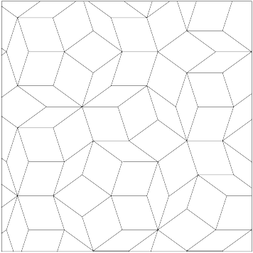
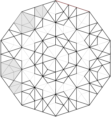
In [1] (1990), I studied with M Baake, M Schlottmann and D Zeidler
the root lattice ![]() in 4-dimensional space. We showed that the projection of 2D Voronoi boundaries
yields the Penrose rhombus tiling Fig. 7, and the dual projection of Delone boundaries yields the
Tübingen triangle tiling Fig 8. These tilings were used to model decagonal quasicrystals [31], [32]
and were related to the Burkov model.
in 4-dimensional space. We showed that the projection of 2D Voronoi boundaries
yields the Penrose rhombus tiling Fig. 7, and the dual projection of Delone boundaries yields the
Tübingen triangle tiling Fig 8. These tilings were used to model decagonal quasicrystals [31], [32]
and were related to the Burkov model.
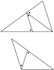
The lattice ![]() also
has a scaling symmetry [1]. The two dual tilings
also
has a scaling symmetry [1]. The two dual tilings ![]() ,
,
![]() admit two inequivalent Robinson-decompositions
into triangles of the shapes appearing in Fig. 8.
From the scaling symmetry there result two different
stone-inflations of these triangular tilings. The stone-inflation for the Penrose tiling is shown in Fig. 9.
This stone inflation
can be used to construct
quasiperiodic
wavelets.
The details are given in [33].
admit two inequivalent Robinson-decompositions
into triangles of the shapes appearing in Fig. 8.
From the scaling symmetry there result two different
stone-inflations of these triangular tilings. The stone-inflation for the Penrose tiling is shown in Fig. 9.
This stone inflation
can be used to construct
quasiperiodic
wavelets.
The details are given in [33].
Work on icosahedral projections and tilings was extended with Z Papadopolos and D Zeidler
in [29] (1992) by analyzing the root lattice ![]() , compare
[8], also denoted as the face-centered
hypercubic lattice in 6 dimensions. This lattice is inequivalent to the
lattice
, compare
[8], also denoted as the face-centered
hypercubic lattice in 6 dimensions. This lattice is inequivalent to the
lattice ![]() . The lattice
. The lattice ![]() can be identified by indexing its diffraction pattern which belongs to its reciprocal lattice, the so called body-centered
hypercubic lattice.
The lattice
can be identified by indexing its diffraction pattern which belongs to its reciprocal lattice, the so called body-centered
hypercubic lattice.
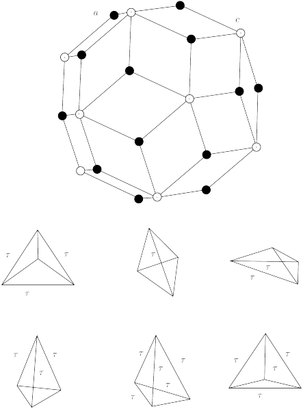
The lattice ![]() occurs in stable phases of
occurs in stable phases of ![]() . We constructed the six tiles for both the
Voronoi- and Delone-based tilings
. We constructed the six tiles for both the
Voronoi- and Delone-based tilings ![]() and
and ![]() .
.
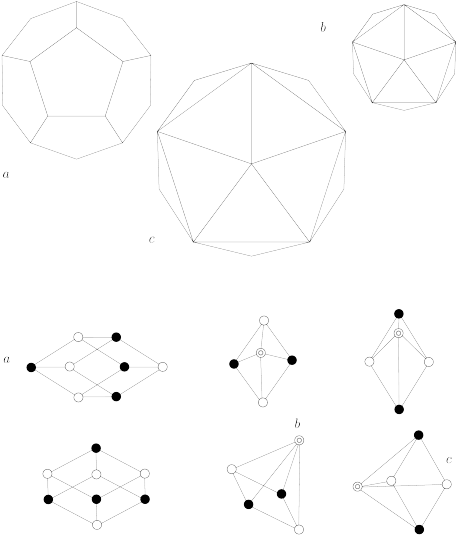
The lattice has three types ![]() of translational inequivalent holes, that is, vertices of its
Voronoi cells, and hence three types of dual Delone cells.
Under icosahedral projection, the tiling
of translational inequivalent holes, that is, vertices of its
Voronoi cells, and hence three types of dual Delone cells.
Under icosahedral projection, the tiling ![]() has the six projections of the 3-boundaries of Voronoi cells as
tiles. These are shown in Fig. 10.
We showed in [30] that the tiling
has the six projections of the 3-boundaries of Voronoi cells as
tiles. These are shown in Fig. 10.
We showed in [30] that the tiling ![]() is equivalent to a tiling constructed
with methods of scaling by Danzer [9]. This tiling in turn is related
to a tiling constructed by Levine and Steinhardt [44], [45]
which in this way is shown to belong to the
is equivalent to a tiling constructed
with methods of scaling by Danzer [9]. This tiling in turn is related
to a tiling constructed by Levine and Steinhardt [44], [45]
which in this way is shown to belong to the ![]() module.
module.